10. Single-Photon Double-Slit Build-up
Module
Particle Nature of Light · Experiment 3
Try it live
Explore this on the interactive simulator with real-time sliders and graphs: 🔬 Launch in Simulator
Aim
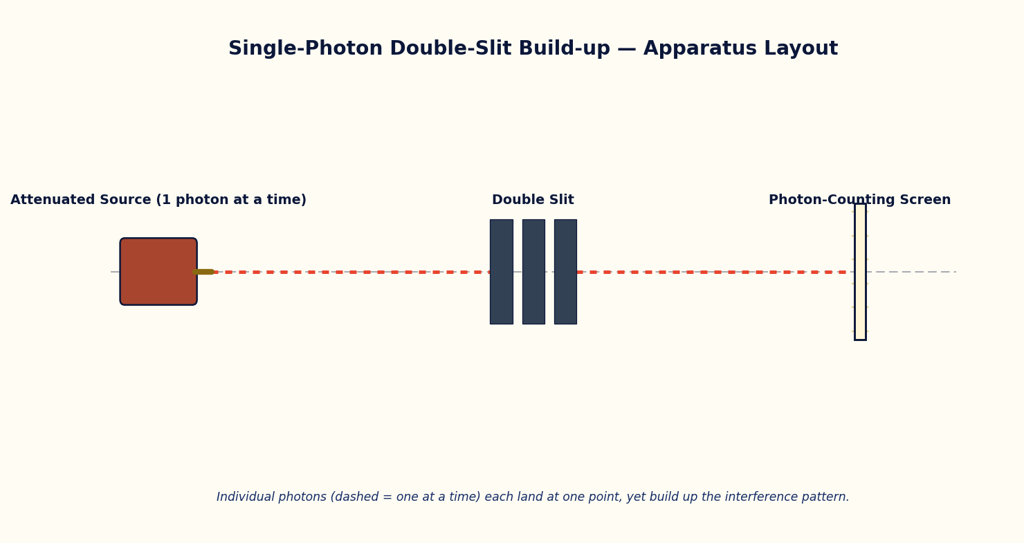
To observe the statistical build-up of an interference pattern from individually detected photons sent through a double slit one at a time, demonstrating wave–particle duality.
Theoretical Background
If photons are sent through a double slit one at a time — so rarely that at most one photon is ever in transit — each photon is still detected as a single, localized point on the screen, exactly as a classical particle would be. There is no way to predict in advance exactly where any individual photon will land.
However, after a large number of such individual detection events accumulate, the resulting pattern of dots is not uniform: it reproduces the same fringe pattern (bright and dark bands) predicted by classical wave interference, with the probability of a photon landing at a given point proportional to the classical intensity, I ∝ cos²(...), of the two-slit pattern at that point.
This experiment shows that no single photon 'knows' about the emerging pattern, nor does it travel through only one slit in the classical sense — the interference pattern is a statistical property that emerges only over many independent, individually-particle-like detection events, encapsulating the essential mystery of wave–particle duality.
Governing Formulas
Probability density (two-slit):
Simulator Controls
| Control | Symbol | Range | Unit |
|---|---|---|---|
| Photon arrival rate | — | 1 – 60 | photons/sec |
Procedure
- Set a low photon arrival rate and start the simulation; observe individual dots appearing at random-looking positions on the screen.
- Let the simulation run and record the number of detected photons at regular intervals (e.g. every 100, 500, 2000 counts).
- At each recorded interval, note (qualitatively or by pixel count binning) whether a fringe pattern is beginning to emerge from the scatter of dots.
- Repeat at a higher arrival rate and confirm that the same final pattern emerges, only more quickly in wall-clock time.
Observation Table
Table: Emergence of the interference pattern with increasing photon count
| S. No. | Total photons detected | Pattern visibility (none / faint / clear fringes) |
|---|---|---|
| 1 | ||
| 2 | ||
| 3 | ||
| 4 | ||
| 5 | ||
| 6 |
Graph
Plot Fringe visibility / contrast (qualitative or measured) (y-axis) against Number of photons detected (log scale) (x-axis).
Expected trend: visibility rising from near-zero (few photons) toward the classical interference contrast (many photons).
Build-up curve: fringe contrast vs cumulative photon count
Calculation
- If a horizontal intensity histogram is exported at each interval, compute the visibility V = (Imax − Imin)/(Imax + Imin) at each stage.
- Plot V against the cumulative photon count and note the count at which V approaches its asymptotic (classical) value.
Result
Table: Fringe visibility versus accumulated photon count
| Photon count | Estimated visibility V |
|---|---|
| 1 | |
| 2 | |
| 3 |
Maximum Permissible Error
This experiment is a qualitative demonstration, not an instrumental measurement — its natural 'error' is the statistical counting uncertainty of accumulating discrete photon detection events, which shrinks as more photons are collected.
Precautions
- Do not judge the pattern from too few detections — early dots always look random regardless of the eventual pattern.
- Keep the arrival rate low enough (conceptually) that at most one photon is 'in flight' at a time, consistent with the single-photon interpretation.
Self-Check Quiz
1. When a single photon is sent through the double slit, where does it land on the screen?
- A) Always exactly at the centre
- B) Spread out continuously like a wave, never at a single point
- C) At one single, localized point — exactly like a classical particle
- D) It doesn't land anywhere unless many photons are sent together
Answer: C — Every individual detection event is a single localized spot — the particle-like behaviour is seen event by event.
2. After thousands of individual photons accumulate one at a time, the resulting pattern of dots:
- A) Is completely random with no structure
- B) Reproduces the classical two-slit interference fringe pattern
- C) Shows only a single-slit pattern
- D) Is uniform across the whole screen
Answer: B — This is the heart of wave–particle duality: individually particle-like detections build up a wave-like interference pattern over many trials.
3. The probability of a photon landing at position y is proportional to:
- A) y itself
- B) cos²(πdy/λD), the same intensity distribution predicted by classical wave interference
- C) A constant, independent of y
- D) 1/y²
Answer: B — P(y) ∝ cos²(πdy/λD) — the quantum probability density exactly matches the classical intensity pattern.
4. Why is it essential that photons are sent 'so rarely that at most one is ever in transit'?
- A) To save laser power
- B) To rule out the possibility that photons are interfering with each other, proving each photon somehow 'interferes with itself'
- C) It isn't essential — the result would be the same either way
- D) To make the experiment run faster
Answer: B — With only one photon in the apparatus at a time, no classical interaction between photons is possible, showing the interference pattern is a single-photon phenomenon.
Viva-Voce Questions
- Does an individual photon pass through one slit or both? What does this experiment tell us about that question?
- How does this experiment settle the wave-versus-particle debate about the nature of light?
- How can an interference pattern build up even when photons are sent through the apparatus one at a time?
- What happens to the interference pattern if a detector is placed at one slit to determine which slit each photon passed through?
- What does this experiment demonstrate about the wave–particle duality of light?
- Why can we not predict exactly where a single photon will land on the screen, only its probability distribution?
- How does the accumulated pattern from many single photons compare with the classical double-slit fringe pattern?