Magnetic Field on the Axis of a Circular Coil & Helmholtz Coils¶

Apparatus layout diagram for this experiment

Labelled apparatus layout — original illustration prepared for this guide (not a photograph). See the drag-to-rotate 3-D schematic above for a spatial view of the same setup.

3-D apparatus schematic · drag to rotate, scroll to zoom · A single virtual circular coil (adjustable R, N, I) with an axial field probe, and a switchable Helmholtz-pair configuration with adjustable coil separation, plotting B(x) along the common axis.

Aim¶

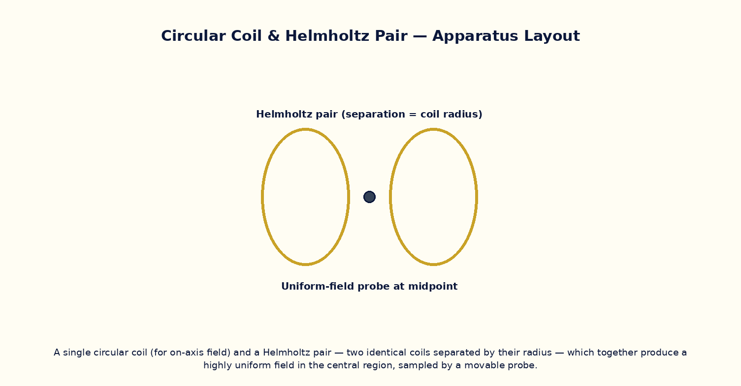
To study the magnetic field along the axis of a single circular current loop, locate the point of maximum field, and demonstrate how a Helmholtz pair produces a highly uniform field at its centre.

Theoretical Background¶

The magnetic field on the axis of a circular coil of radius R and N turns carrying current I, at an axial distance x from its centre, is B(x) = μ₀NIR² / [2(R²+x²)^(3/2)]. At the centre (x = 0) this reduces to B₀ = μ₀NI/2R, the maximum value. Two identical coils placed coaxially and separated by a distance equal to their common radius R (the 'Helmholtz' condition) produce a combined field whose second derivative with respect to x vanishes at the midpoint — making the field remarkably uniform over a useful volume between the coils, which is why Helmholtz coils are the standard tool for producing a known, controllable, uniform field for calibrating magnetometers and cancelling the Earth's field in sensitive experiments.

Governing Formula¶

\[ B(x) = μ₀ N I R² / [2(R² + x²)^{3/2}] \]

Symbol	Meaning
B(x)	axial field at distance x from the coil centre (T)
N	number of turns
I	current (A)
R	coil radius (m)
x	axial distance from the coil's centre (m)

Interactive Controls¶

Launch the simulator and use the following controls on the Magnetic Field on the Axis of a Circular Coil & Helmholtz Coils panel:

Control	Symbol	Range	Default
Coil radius	R	5–30 cm	10 cm
Number of turns	N	1–500	100
Current	I	0.1–5 A	1 A
Axial distance from centre	x	-30–30 cm	0 cm
Helmholtz coil separation (mode 2)	d	5–30 cm	10 cm

Procedure¶

For a single coil, sweep x from −30 cm to +30 cm and plot B(x); verify the peak occurs at x = 0 with value μ₀NI/2R.
Verify B(0) ∝ N and B(0) ∝ I by varying each independently.
Switch to the Helmholtz configuration with separation d = R and plot the combined field along the axis; note the flat region near the midpoint.
Change the separation away from d = R (e.g. d = 0.5R or 2R) and observe the field profile becoming non-uniform (dip or double-hump).
Estimate the useful 'uniform-field volume' (region where B stays within 1% of the central value) for the ideal Helmholtz separation.
Compute the theoretical central field of the Helmholtz pair and compare with the simulator's numerically-integrated value.

Observation Table¶

| S. No. | x (cm) | R (cm) | N | I (A) | Field B (×10⁻⁴ T) | |---|---|---|---|---|---|| | | | | | | | | | | | | | | | | | | | | | | | | | | | | | | | | | | |

Graph¶

B(x) Along the Coil Axis — peak at x=0 for single coil; flat-top for Helmholtz pair

15×15 grid — choose your own scale per square; plot from your observation table. Expected trend: peak at x=0 for single coil; flat-top for Helmholtz pair

Calculations¶

Use the governing formula above with your tabulated observations to compute the required result for each row. Show at least one complete sample calculation with units.

Result¶

| Configuration | Field uniformity (ΔB/B over ±2 cm) | Optimum separation d | Remarks | |---|---|---|---|| | | | | |

Precautions¶

Keep R, N and I fixed while sweeping x to isolate the axial-distance dependence cleanly.
For the Helmholtz study, change only the coil separation d between runs, not R, N or I.
Note the field falls off increasingly steeply for |x| ≫ R; keep this in mind when defining the 'uniform region'.
Remember the Helmholtz condition (d = R) is optimal only for the specific criterion of a vanishing second derivative at the centre — other criteria give slightly different optimal spacings.

Maximum Permissible Error¶

\[ ΔB₀/B₀ = ΔN/N + ΔI/I + ΔR/R \]

B₀ = μ₀NI/2R at the coil centre is a simple product/quotient, so fractional errors add.

Viva-Voce Questions¶

Derive the on-axis field of a circular current loop starting from the Biot–Savart law.
At what axial distance does B(x) fall to half its central value, for a single coil?
Why is the Helmholtz coil separation chosen equal to the coil radius?
What physical quantity being zero at the midpoint makes the Helmholtz field so uniform there?
How would you use a Helmholtz pair to cancel the Earth's magnetic field in a sensitive experiment?
Compare the on-axis field of a coil with that of a long solenoid — under what condition does one reduce to the other?