LCR Series Resonance & Quality Factor (Q)
Aim
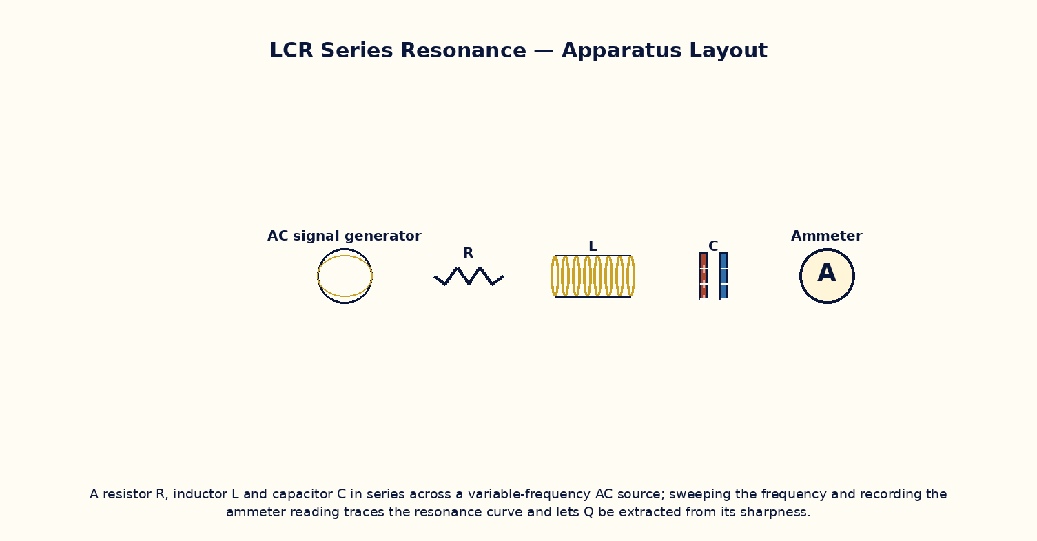
To study the resonance behaviour of a series LCR circuit driven by an AC source, locate the resonant frequency, and determine the quality factor from the sharpness of the resonance curve.
Theoretical Background
In a series LCR circuit driven by a sinusoidal source of angular frequency ω, the impedance is Z = √[R² + (ωL − 1/ωC)²]. The current amplitude I(ω) = V₀/Z is maximum when the reactive term vanishes, at the resonant angular frequency ω₀ = 1/√(LC), where the impedance reduces to purely R and the circuit behaves resistively with the largest possible current. The sharpness of the resonance peak is characterised by the quality factor Q = ω₀L/R = (1/R)√(L/C) = ω₀/Δω, where Δω is the full width of the resonance curve at half the maximum power (equivalently, at I = I_max/√2). A higher Q means a lower R relative to √(L/C), giving a narrower, taller resonance peak and better frequency selectivity, as exploited in radio tuning circuits.
Governing Formula
| Symbol | Meaning |
|---|---|
| ω₀ | resonant angular frequency (rad/s) |
| L | inductance (H) |
| C | capacitance (F) |
| R | resistance (Ω) |
| Q | quality factor (dimensionless) |
Interactive Controls
Launch the simulator and use the following controls on the LCR Series Resonance & Quality Factor (Q) panel:
| Control | Symbol | Range | Default |
|---|---|---|---|
| Resistance | R | 1–200 Ω | 20 Ω |
| Inductance | L | 1–500 mH | 100 mH |
| Capacitance | C | 0.1–10 μF | 1 μF |
| Source amplitude | V₀ | 1–20 V | 10 V |
| Drive frequency | f | 10–5000 Hz | 500 Hz |
Procedure
- Sweep the drive frequency f across a wide range and plot the current amplitude I(f); locate the peak and compare with f₀ = 1/(2π√LC).
- Read off the half-power frequencies (where I = I_max/√2) and compute the bandwidth Δf; hence determine Q = f₀/Δf.
- Increase R (keeping L, C fixed) and observe the resonance peak becoming shorter and broader; verify Q decreases as expected.
- Vary L and C while keeping their product LC fixed (so f₀ is unchanged) and observe how the peak height and width change with √(L/C).
- At resonance, verify that the voltage across L and across C individually can each exceed the source voltage V₀, while remaining 180° out of phase with each other.
- Compute Q by two independent methods — from the bandwidth, and from Q = ω₀L/R — and compare.
Observation Table
| S. No. | R (Ω) | L (mH) | C (μF) | Frequency f (Hz) | Current amplitude I (mA) | |---|---|---|---|---|---|| | | | | | | | | | | | | | | | | | | | | | | | | | | | | | | | | | | |
Graph
Resonance Curve: Current vs Frequency — peak at f₀; width sets Q
Calculations
Use the governing formula above with your tabulated observations to compute the required result for each row. Show at least one complete sample calculation with units.
Result
| Quantity | Measured value | Calculated value | % deviation | |---|---|---|---|| | | | | |
Precautions
- Sweep frequency finely (small steps) near resonance, since the peak can be narrow for high-Q circuits.
- Keep the source amplitude V₀ fixed throughout a frequency sweep.
- Vary only one of R, L, C at a time when studying their individual effects on the resonance curve.
- Remember the individual voltages across L and C can exceed the source voltage at resonance — this is expected, not an error.
Maximum Permissible Error
f₀ = 1/(2π√LC) involves a square root of the product LC, halving the summed fractional errors.
Viva-Voce Questions
- Derive the resonant frequency of a series LCR circuit from its impedance expression.
- Define quality factor Q in at least two equivalent ways and show they are consistent.
- Why can the voltage across the inductor or capacitor individually exceed the applied source voltage at resonance?
- How does increasing R affect the sharpness and height of the resonance curve?
- Compare series and parallel LCR resonance — which one gives minimum impedance and which gives maximum impedance at resonance?
- Explain how this resonance principle is used in radio-frequency tuning circuits.