Rectangular Waveguide — TE₁₀ Mode & Cutoff Frequency
Aim
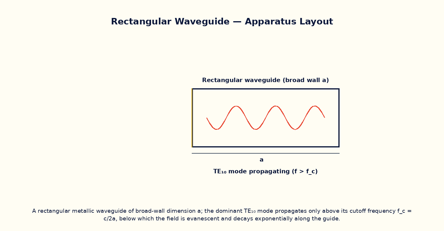
To compute the cutoff frequency of the dominant TE₁₀ mode of a rectangular waveguide from its broad-wall dimension, and determine whether a given signal frequency will propagate or be evanescently attenuated.
Theoretical Background
Unlike a coaxial cable or a simple pair of wires, a hollow rectangular metallic waveguide cannot support a signal at every frequency: for each mode (a particular transverse field pattern satisfying the boundary conditions on the conducting walls), there is a minimum cutoff frequency f_c below which the wave cannot propagate and instead decays exponentially with distance along the guide (an evanescent wave). The dominant, lowest-cutoff mode of a rectangular guide is TE₁₀, whose cutoff frequency depends only on the guide's broad-wall dimension a: f_c = c/(2a). Operating well above cutoff (but below the cutoff of the next higher mode) ensures single-mode propagation with low loss, which is why waveguide dimensions are chosen very deliberately in radar, satellite and microwave engineering to match the intended operating frequency band.
Governing Formula
| Symbol | Meaning |
|---|---|
| f_c | cutoff frequency of the TE₁₀ mode (Hz) |
| c | speed of light in vacuum |
| a | waveguide broad-wall (longer transverse) dimension (m) |
| f | actual signal frequency being tested (Hz) |
Interactive Controls
Launch the simulator and use the following controls on the Rectangular Waveguide — TE₁₀ Mode & Cutoff Frequency panel:
| Control | Symbol | Range | Default |
|---|---|---|---|
| Waveguide broad-wall dimension | a | 1–10 cm | 2.29 cm |
| Signal frequency | f | 1–20 GHz | 9 GHz |
Procedure
- Fix a = 2.29 cm (a standard X-band waveguide dimension) and compute f_c.
- Vary the signal frequency f from 1 GHz to 20 GHz and, for each value, note whether the simulator reports propagation or evanescent attenuation.
- Vary the broad-wall dimension a and observe how f_c shifts; verify f_c ∝ 1/a by plotting f_c versus 1/a.
- Determine the range of a for which a fixed signal frequency (e.g. 9 GHz) propagates in the dominant mode only (i.e. above the TE₁₀ cutoff but below the next mode's cutoff, roughly 2f_c).
- Discuss why waveguides are generally unsuitable for carrying signals at frequencies much below the microwave range (the required a would become impractically large).
Observation Table
| S. No. | a (cm) | f_c (GHz) | f tested (GHz) | Propagates? (Y/N) | |---|---|---|---|---|| | | | | | | | | | | | | | | | | | | | | | | | | | | | | | |
Graph
Cutoff frequency f_c vs 1/a
Calculations
Use the governing formula above with your tabulated observations to compute the required result for each row. Show at least one complete sample calculation with units.
Result
| Quantity | Slope of f_c vs 1/a (→ c/2) | Expected value | % deviation | |---|---|---|---|| | | | | |
Precautions
- Remember the cutoff condition depends only on the broad-wall dimension a for the TE₁₀ mode, not on the narrower dimension b.
- Operate the guide below the cutoff of the next higher-order mode to avoid multi-mode propagation.
- Change only a or f at a time when tabulating.
- Treat the waveguide walls as perfectly conducting for this idealised cutoff calculation.
Maximum Permissible Error
f_c = c/(2a) is inversely proportional to a alone, so its fractional error equals that of the measured dimension a.
Viva-Voce Questions
- Explain physically why a hollow waveguide has a cutoff frequency while a coaxial cable does not.
- Derive the TE₁₀ cutoff frequency from the boundary conditions on the waveguide walls.
- What happens to a signal launched below the cutoff frequency?
- Why is TE₁₀ called the 'dominant mode'?
- How would you choose waveguide dimensions for an X-band radar system operating near 9–10 GHz?