Charge Distribution on Conductors & the Van de Graaff Generator
Aim
To study how charge distributes itself over the surface of conductors of different shapes at electrostatic equilibrium, and to understand the principle of the Van de Graaff generator for building up very high potentials.
Theoretical Background
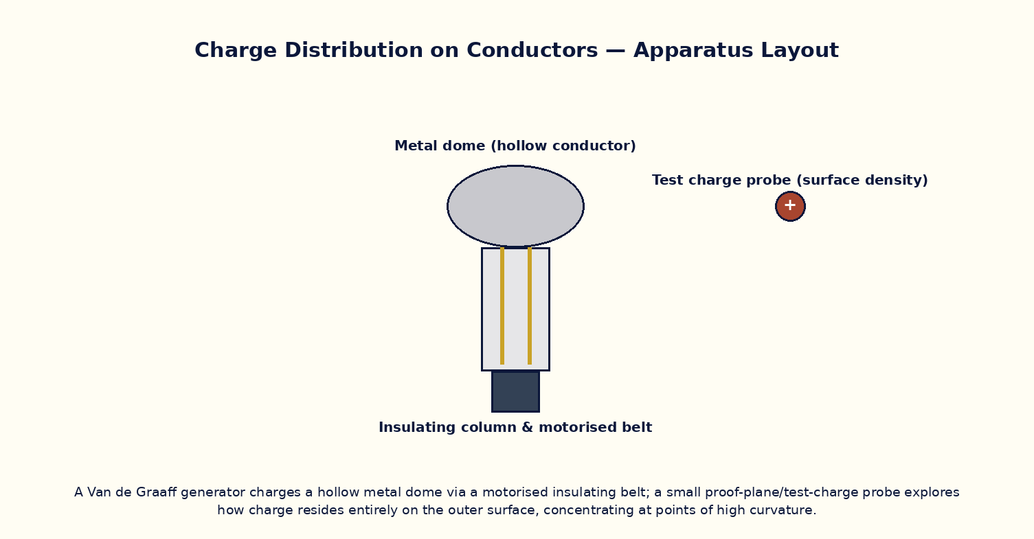
At electrostatic equilibrium, the electric field inside a conductor is zero and any excess charge resides entirely on its outer surface, arranging itself so the surface is an equipotential. Surface charge density σ is not uniform for a non-spherical conductor — it is highest where the surface curvature is greatest (sharp points and edges), which is why the field just outside a sharp point (E = σ/ε₀) can become large enough to ionize the surrounding air ('action at points', used in lightning rods and van de Graaff brush discharge). A Van de Graaff generator exploits the fact that if a charged conductor is brought inside a larger hollow conductor and touched to its inner surface, all its charge transfers to the outer surface of the larger conductor, however much charge the outer shell already carries — the potential can therefore be raised indefinitely by repeatedly carrying small charges up an insulating belt into the hollow dome.
Governing Formula
| Symbol | Meaning |
|---|---|
| V_dome | potential of the charged spherical dome (V) |
| Q | total charge delivered to the dome (C) |
| R | radius of the dome (m) |
| σ | local surface charge density (C/m²) |
Interactive Controls
Launch the simulator and use the following controls on the Charge Distribution on Conductors & the Van de Graaff Generator panel:
| Control | Symbol | Range | Default |
|---|---|---|---|
| Dome radius | R | 10–50 cm | 25 cm |
| Belt charging rate | rate | 1–20 nC/s | 5 nC/s |
| Charging time | t | 0–60 s | 20 s |
| Test conductor tip radius (for point-discharge study) | r_tip | 0.5–20 mm | 2 mm |
Procedure
- Charge the Van de Graaff dome for increasing durations and plot dome potential V versus charging time t; verify V ∝ t (constant charging rate).
- For a fixed total charge, vary the dome radius R and verify V ∝ 1/R.
- Observe the surface-charge heat-map on an ellipsoidal conductor and note that charge density is highest at the sharper end.
- Reduce the tip radius of a test conductor and note the field at the tip rising as 1/r_tip until corona discharge (visualised as a glow) sets in.
- Verify numerically that the field just inside the conductor's surface is zero at every point, regardless of shape.
- Bring a small pre-charged test sphere inside the dome and touch it to the inner wall; confirm all of its charge transfers to the dome's outer surface.
Observation Table
| S. No. | Charging time t (s) | Rate (nC/s) | Total charge Q (nC) | Dome radius R (cm) | Dome potential V (kV) | |---|---|---|---|---|---|| | | | | | | | | | | | | | | | | | | | | | | | | | | | | | | | | | | |
Graph
Dome Potential vs Charging Time — V ∝ t at constant charging rate
Calculations
Use the governing formula above with your tabulated observations to compute the required result for each row. Show at least one complete sample calculation with units.
Result
| Quantity studied | Observed trend | Theoretical prediction | Agreement | |---|---|---|---|| | | | | |
Precautions
- Keep the charging rate constant while studying the V–t relationship; vary only one control at a time.
- Note that real Van de Graaff generators are limited by the dielectric breakdown of surrounding air, not by the belt mechanism itself.
- Remember the field inside any conductor is exactly zero at equilibrium — a common source of confusion is expecting a small residual field.
- When studying the sharp-point tip, understand this is an idealization; real points are never perfectly sharp.
Maximum Permissible Error
V = kQ/R with Q = rate×t (charging rate times time), so fractional errors in rate, time and R all add.
Viva-Voce Questions
- Why must the electric field inside a conductor in electrostatic equilibrium be zero?
- Explain why charge density is greatest at the sharpest points of a charged conductor.
- How does a Van de Graaff generator manage to raise the dome to a very high potential regardless of the charge already present on it?
- What is corona discharge and why does it limit the maximum achievable potential?
- State the boundary condition on E just outside a charged conductor's surface in terms of σ.
- Why is the interior of a hollow charged conductor field-free even if the shell is not spherical (Faraday cage)?