Eddy-Current Damping — Lenz's Law Braking¶

Apparatus layout diagram for this experiment

Labelled apparatus layout — original illustration prepared for this guide (not a photograph). See the drag-to-rotate 3-D schematic above for a spatial view of the same setup.

3-D apparatus schematic · drag to rotate, scroll to zoom · A conducting plate moves with velocity v through a localised magnetic field region; the eddy currents induced in the plate oppose the field change (Lenz's law), producing a velocity-dependent retarding force.

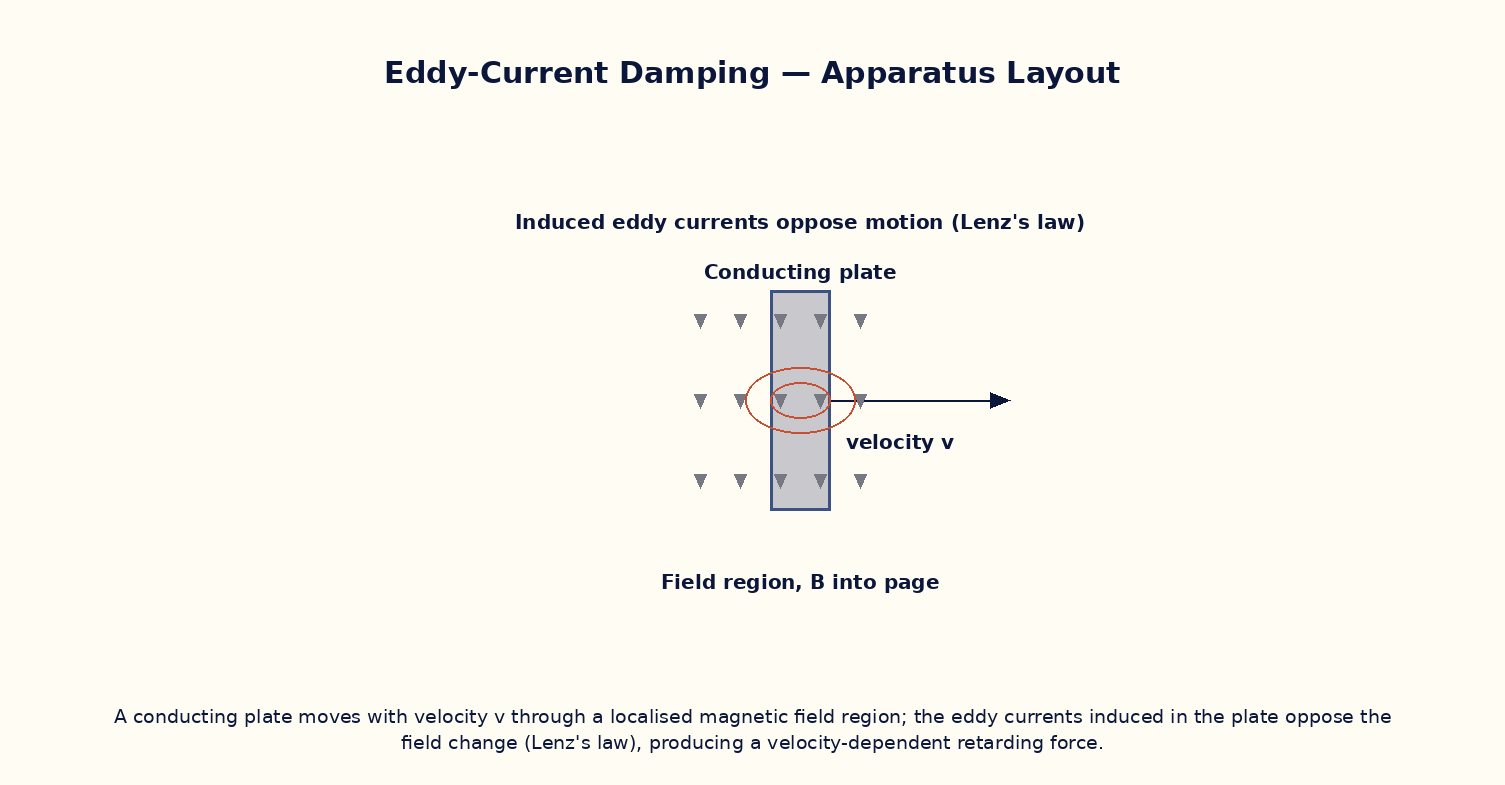
Aim¶

To model the retarding force experienced by a conducting plate moving through a non-uniform magnetic field due to induced eddy currents, and study its dependence on conductivity, plate thickness, speed and field strength.

Theoretical Background¶

When a solid conductor moves through a region of non-uniform magnetic field (or experiences a changing flux), Faraday's law induces circulating eddy currents within the bulk of the material, not just in a single wire loop. By Lenz's law, these eddy currents flow in whatever direction opposes the change that created them, which means they exert a retarding (braking) force on the moving conductor — converting its kinetic energy into resistive (I²R) heating within the material itself. This eddy-current braking effect grows with the conductor's electrical conductivity, its speed through the field, and the square of the field strength, and is exploited in applications ranging from magnetic braking systems in trains and roller coasters to the damping mechanisms of sensitive analog galvanometers and electricity meters.

Governing Formula¶

\[ F_{eddy} \propto \sigma\, t\, B^2\, v\, w^2 \]

Symbol	Meaning
F_eddy	eddy-current retarding force (N)
σ	electrical conductivity of the plate (S/m)
t	plate thickness (m)
B	magnetic flux density in the field region (T)
v	plate velocity through the field (m/s)
w	characteristic width of the induced current loops (m)

Interactive Controls¶

Launch the simulator and use the following controls on the Eddy-Current Damping — Lenz's Law Braking panel:

Control	Symbol	Range	Default
Magnetic flux density	B	10–500 mT	200 mT
Plate velocity	v	0.1–10 m/s	2 m/s
Plate conductivity	σ	1–60 ×10⁶ S/m	35 ×10⁶ S/m
Plate thickness	t	0.5–10 mm	3 mm

Procedure¶

Fix B, σ, t at their default values and vary v from 0.1 to 10 m/s, recording the retarding force F.
Plot F versus v and verify a straight line through the origin, confirming F ∝ v at fixed field and material.
Fix v and vary B, and verify that F ∝ B² by plotting F versus B².
Fix B and v and vary the plate conductivity σ (e.g. comparing an aluminium-like and a copper-like value), and verify F ∝ σ.
Vary the plate thickness t and verify F ∝ t; discuss why a thicker plate experiences greater eddy-current braking.

Observation Table¶

| S. No. | v (m/s) | B (mT) | σ (×10⁶ S/m) | t (mm) | F (mN) | |---|---|---|---|---|---|| | | | | | | | | | | | | | | | | | | | | | | | | | | | | | | | | | | |

Graph¶

Retarding force F vs velocity v

Calculations¶

Use the governing formula above with your tabulated observations to compute the required result for each row. Show at least one complete sample calculation with units.

Result¶

| Quantity | Slope of F vs v | Expected value | % deviation | |---|---|---|---|| | | | | |

Precautions¶

Keep the field region localised (non-uniform) — a perfectly uniform infinite field produces no net eddy-current braking on a plate moving through it.
Vary only one of B, v, σ, t at a time while tabulating the others.
Note that F ∝ B², so small errors in B are doubled in their effect on the computed force.
Distinguish eddy-current braking (a bulk, continuous-medium effect) from the induced EMF in a single discrete loop (Faraday's law experiment).

Maximum Permissible Error¶

\[ \dfrac{\Delta F}{F} = \dfrac{\Delta\sigma}{\sigma} + \dfrac{\Delta t}{t} + 2\dfrac{\Delta B}{B} + \dfrac{\Delta v}{v} \]

F ∝ σtB²v has B squared, so its fractional error contributes twice to the total.

Viva-Voce Questions¶

Explain, using Lenz's law, why eddy currents always oppose the motion that creates them.
Why does eddy-current braking require a non-uniform (spatially varying) field rather than a uniform one?
Where does the kinetic energy lost by the moving conductor ultimately go?
Name two practical applications of eddy-current damping.
Why are laminated cores (thin insulated sheets) used in transformers to reduce eddy-current losses?