Maxwell's Equations & Plane Electromagnetic Wave Solutions¶

Apparatus layout diagram for this experiment

Labelled apparatus layout — original illustration prepared for this guide (not a photograph). See the drag-to-rotate 3-D schematic above for a spatial view of the same setup.

3-D apparatus schematic · drag to rotate, scroll to zoom · A virtual 3-D animated E and B field visualiser for a plane wave propagating along z, with adjustable frequency and amplitude, and a toggle to independently vary E-field and B-field phase/amplitude to see how the wave 'breaks' if Maxwell's relations are violated.

Aim¶

To explore how Maxwell's four equations, together, predict self-sustaining transverse electromagnetic waves in free space, and to verify the relations between E, B, their phase, and the speed of light.

Theoretical Background¶

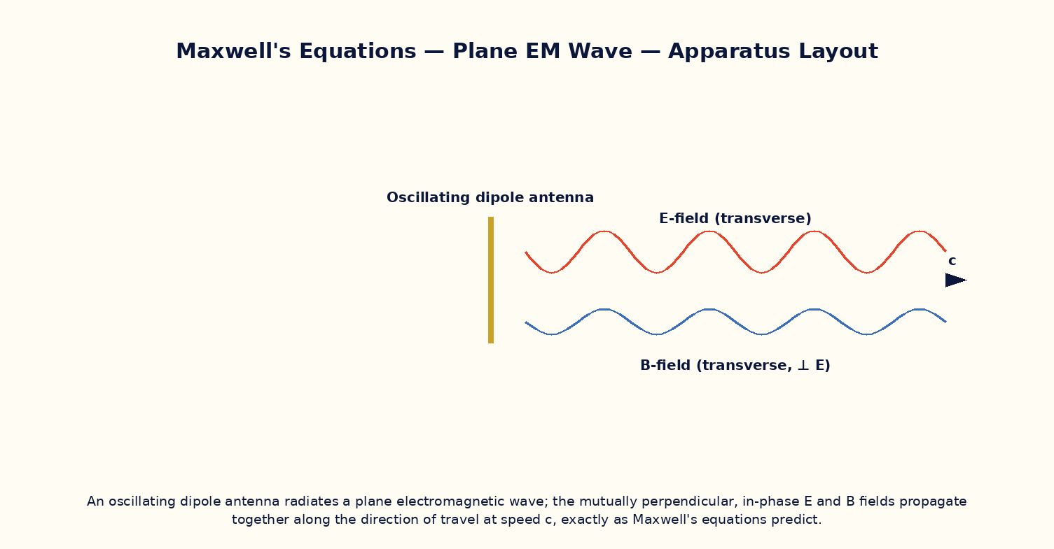
Maxwell's equations in free space (no charges or currents) are ∇·E = 0, ∇·B = 0, ∇×E = −∂B/∂t, and ∇×B = μ₀ε₀∂E/∂t. Combining the curl equations by taking the curl of one and substituting the other yields a wave equation ∇²E = μ₀ε₀∂²E/∂t² (and similarly for B), whose solutions are transverse waves travelling at speed c = 1/√(μ₀ε₀) ≈ 3×10⁸ m/s. For a plane wave travelling along z, E = E₀ sin(kz−ωt) x̂ and B = B₀ sin(kz−ωt) ŷ, with E and B mutually perpendicular, both perpendicular to the direction of propagation, oscillating exactly in phase, and related in magnitude by B₀ = E₀/c at every instant. This is the theoretical foundation for all of classical optics, radio, and wireless communication.

Governing Formula¶

\[ c = 1/√(μ₀ε₀), E₀/B₀ = c, E ⊥ B ⊥ direction of propagation \]

Symbol	Meaning
c	speed of light in vacuum (m/s)
μ₀	permeability of free space
ε₀	permittivity of free space
E₀, B₀	peak amplitudes of the electric and magnetic fields

Interactive Controls¶

Launch the simulator and use the following controls on the Maxwell's Equations & Plane Electromagnetic Wave Solutions panel:

Control	Symbol	Range	Default
Wave frequency	f	1–1000 MHz	100 MHz
Electric field amplitude	E₀	1–100 V/m	30 V/m
Artificial E-B phase offset (should be 0 physically)	Δφ	0–90 °	0 °

Procedure¶

Set the phase offset to zero and observe E and B oscillating exactly in phase, perpendicular to each other and to the propagation direction.
Read off B₀ for a chosen E₀ and verify B₀ = E₀/c.
Increase the frequency and verify the wavelength λ = c/f shrinks proportionally while the wave speed itself stays fixed at c.
Artificially introduce a phase offset between E and B using the slider and note this is not a physically realizable free-space plane wave (illustrating why Maxwell's equations force them in phase).
Verify ∇·E = 0 for the plane wave by checking E has no component along its own direction of travel (purely transverse).
Compute the Poynting vector S = E×B/μ₀ direction and confirm it points along the propagation direction, carrying energy forward.

Observation Table¶

| S. No. | Frequency f (MHz) | E₀ (V/m) | Computed B₀ (nT) | Wavelength λ (m) | E₀/B₀ ratio (×10⁸ m/s) | |---|---|---|---|---|---|| | | | | | | | | | | | | | | | | | | | | | | | | | | | | | | | | | | |

Graph¶

E and B Field Snapshot vs Position — E and B in phase, 90° apart in space

15×15 grid — choose your own scale per square; plot from your observation table. Expected trend: E and B in phase, 90° apart in space

Calculations¶

Use the governing formula above with your tabulated observations to compute the required result for each row. Show at least one complete sample calculation with units.

Result¶

| Quantity | Measured value | Theoretical value (c) | % deviation | |---|---|---|---|| | | | | |

Precautions¶

Keep the phase-offset slider at zero except when specifically studying the (unphysical) mismatched case.
Remember E₀/B₀ = c only in SI units with E in V/m and B in tesla — check units carefully when verifying numerically.
Note that both E and B carry energy; the total energy density is shared equally between them in vacuum.
Distinguish the wave's phase velocity (always c in vacuum) from the frequency, which is set by the source.

Maximum Permissible Error¶

\[ ΔB₀/B₀ = ΔE₀/E₀ \]

Since B₀ = E₀/c with c an exact constant, the fractional error in B₀ equals the fractional error in the measured E₀.

Viva-Voce Questions¶

Starting from Maxwell's curl equations, outline the steps to derive the electromagnetic wave equation.
Why must E and B be mutually perpendicular and both transverse to the direction of propagation?
Show dimensionally that 1/√(μ₀ε₀) has the units of speed.
What physical role does Maxwell's displacement current term play in predicting wave propagation?
How is the Poynting vector defined, and what does it represent physically?
Why was the prediction of electromagnetic waves by Maxwell considered one of the great unifications in physics?