Multipole Expansion — Linear Electric Quadrupole¶

Apparatus layout diagram for this experiment

Labelled apparatus layout — original illustration prepared for this guide (not a photograph). See the drag-to-rotate 3-D schematic above for a spatial view of the same setup.

3-D apparatus schematic · drag to rotate, scroll to zoom · Three collinear charges +q, −2q, +q (a linear quadrupole) with a distant field point P on the axis; the simulator isolates the pure quadrupole potential term, which falls off as 1/r³.

Aim¶

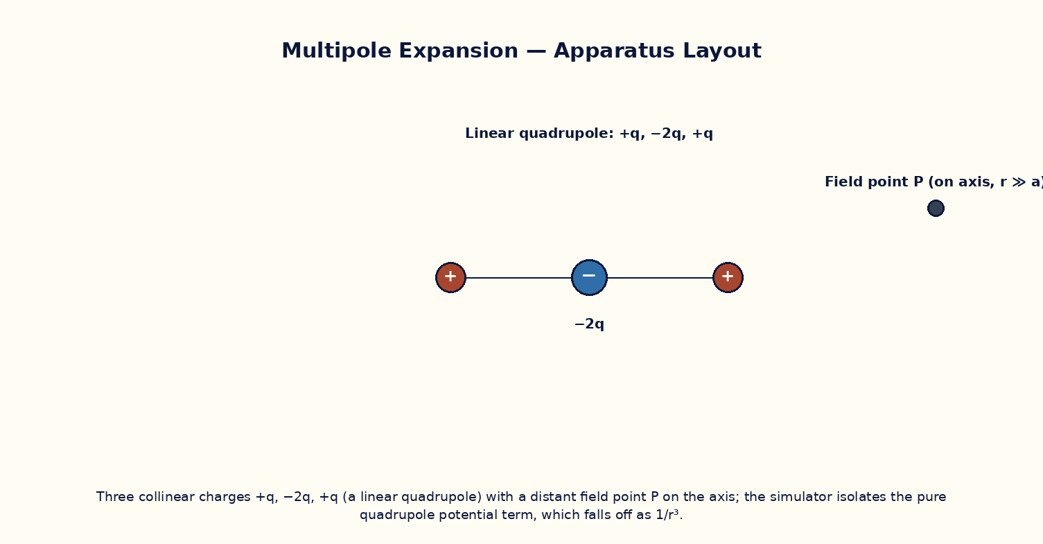
To compute the far-field electric potential of a linear quadrupole and verify its characteristic 1/r³ fall-off, distinguishing it from the 1/r monopole and 1/r² dipole terms of the general multipole expansion.

Theoretical Background¶

The multipole expansion writes the electrostatic potential of any localized charge distribution, viewed from far away, as a sum of terms falling off as successively higher inverse powers of distance: a monopole term (∝1/r, present only if the net charge is non-zero), a dipole term (∝1/r², present if the charge has a net dipole moment even though the total charge is zero), and a quadrupole term (∝1/r³), and so on. A linear quadrupole — charges +q, −2q, +q arranged collinearly with spacing a — has zero net charge and, by symmetry, zero dipole moment, so its leading far-field term is the quadrupole contribution. This configuration models, for example, the charge distribution of a linear symmetric molecule such as CO₂, whose field at large distances is dominated by its quadrupole moment rather than any monopole or dipole term.

Governing Formula¶

\[ V_{quad}(r) = \dfrac{3qa^2}{4\pi\varepsilon_0 r^3} \]

Symbol	Meaning
V	on-axis quadrupole potential at distance r (V)
q	magnitude of the end charges (C)
a	spacing between adjacent charges (m)
r	distance to the field point, r ≫ a

Interactive Controls¶

Launch the simulator and use the following controls on the Multipole Expansion — Linear Electric Quadrupole panel:

Control	Symbol	Range	Default
End charge magnitude	q	1–30 nC	8 nC
Charge spacing	a	0.5–5 cm	2 cm
Field point distance (on axis)	r	10–100 cm	40 cm

Procedure¶

Set q = 8 nC and a = 2 cm, and vary r from 10 cm to 100 cm, recording the computed quadrupole potential.
Plot log V versus log r and verify the slope is −3, confirming the 1/r³ quadrupole fall-off.
Fix r and vary a, verifying that V is proportional to a².
Compare the magnitude of V at a given r with what a simple dipole of moment p = qa would give at the same r, and note how much faster the quadrupole term decays.
Discuss why a genuinely neutral, non-polar linear molecule can still exert a long-range electrostatic influence on a nearby ion.

Observation Table¶

| S. No. | r (cm) | q (nC) | a (cm) | V (×10⁻⁹ V) | log r | log V | |---|---|---|---|---|---|---|| | | | | | | | | | | | | | | | | | | | | | | | | | | | | | | | | | | | | | | | |

Graph¶

log V vs log r (slope method)

Calculations¶

Use the governing formula above with your tabulated observations to compute the required result for each row. Show at least one complete sample calculation with units.

Result¶

| Quantity | Slope of log V vs log r | Expected value | % deviation | |---|---|---|---|| | | | | |

Precautions¶

Keep r large compared with a so the far-field (multipole) approximation remains valid.
Ensure the two end charges are equal in magnitude so the configuration truly has zero net dipole moment.
Take the field point strictly on the axis of the array to use the simplified on-axis formula.
Vary one parameter at a time (q, a, or r) while tabulating.

Maximum Permissible Error¶

\[ \dfrac{\Delta V}{V} = \dfrac{\Delta q}{q} + 2\dfrac{\Delta a}{a} + 3\dfrac{\Delta r}{r} \]

V ∝ qa²/r³ has a squared and r cubed, contributing factors of 2 and 3 respectively to the fractional error.

Viva-Voce Questions¶

Define the electric quadrupole moment and give an example of a real molecule that possesses one.
Why does a linear array of +q, −2q, +q have zero net dipole moment?
Explain, in general terms, why successive multipole terms fall off with increasing powers of 1/r.
How would the far-field potential change if the two end charges were unequal?
What is the physical origin of quadrupole radiation in the time-varying (radiating) case?