Magnetic Hysteresis & the B–H Curve of Ferromagnetic Materials¶

Apparatus layout diagram for this experiment

Labelled apparatus layout — original illustration prepared for this guide (not a photograph). See the drag-to-rotate 3-D schematic above for a spatial view of the same setup.

3-D apparatus schematic · drag to rotate, scroll to zoom · A virtual toroidal sample of selectable ferromagnetic material (soft iron, hard steel, ferrite) wound with a magnetizing coil whose current (hence H) can be cycled, with a live B–H plotter tracing out the hysteresis loop and reporting B_sat, B_r, H_c and loop area.

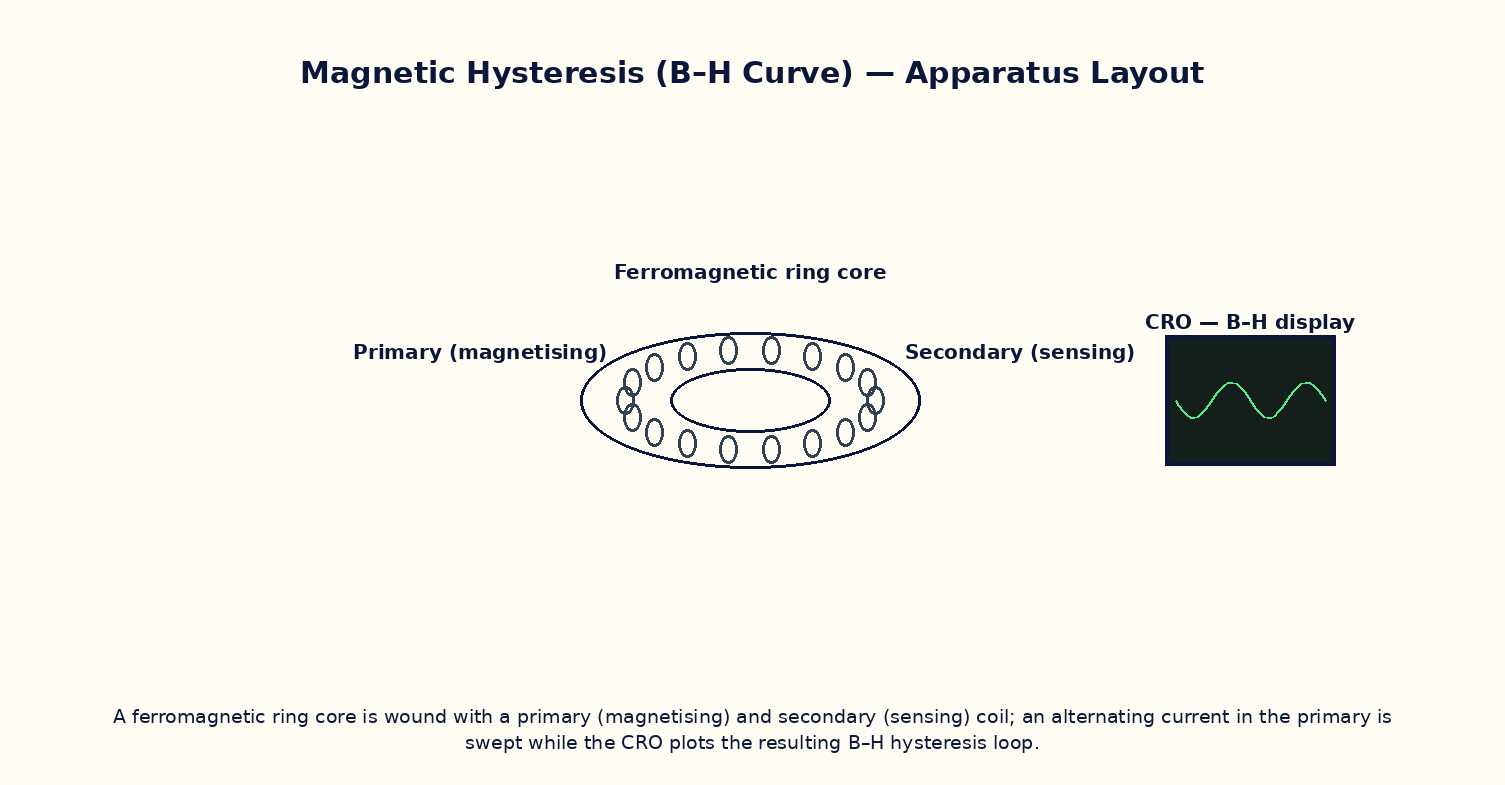
Aim¶

To trace the B–H hysteresis loop of a ferromagnetic material as the applied field H is cycled, and to determine the saturation magnetization, retentivity (remanence), coercivity, and hysteresis energy loss per cycle.

Theoretical Background¶

In a ferromagnetic material, the magnetic flux density B does not respond linearly or reversibly to the applied field H; instead it traces a hysteresis loop B(H) that depends on the material's magnetic history. Starting from an unmagnetized sample and increasing H, B rises along an initial magnetization curve toward saturation B_sat, where nearly all magnetic domains have aligned with the field. Reducing H back to zero leaves a residual flux density called the retentivity (remanence) B_r. Reversing H further, B falls to zero only at a negative field called the coercivity −H_c, the field needed to fully demagnetize the sample. Continuing the cycle traces the full closed loop. The area enclosed by the B–H loop equals the energy dissipated as heat per unit volume per cycle (hysteresis loss), due to irreversible domain-wall motion — which is why transformer cores use 'soft' magnetic materials with narrow loops (low B_r, low H_c, small area) while permanent magnets use 'hard' materials with wide loops (high B_r, high H_c).

Governing Formula¶

\[ H = nI, Hysteresis loss per cycle per unit volume = ∮ H dB (loop area) \]

Symbol	Meaning
H	magnetizing field (A/m)
B	magnetic flux density in the material (T)
B_r	retentivity / remanence (T)
H_c	coercivity (A/m)
B_sat	saturation flux density (T)

Interactive Controls¶

Launch the simulator and use the following controls on the Magnetic Hysteresis & the B–H Curve of Ferromagnetic Materials panel:

Control	Symbol	Range	Default
Material (0=soft iron, 1=ferrite, 2=hard steel)	mat	0–2	0
Peak applied field	H_max	50–2000 A/m	500 A/m
Number of cycles to trace	n	1–5	1

Procedure¶

Starting from an unmagnetized (virgin) sample, increase H from 0 to H_max and trace the initial magnetization curve up to saturation.
Cycle H from +H_max to −H_max and back, tracing the full closed hysteresis loop; read off B_r (at H=0) and H_c (at B=0) from the plot.
Repeat for a 'soft' material (small loop) and a 'hard' material (wide loop) and compare B_r, H_c and loop areas.
Estimate the hysteresis energy loss per cycle per unit volume by numerically computing the enclosed loop area, ∮H dB.
Reduce H_max below saturation and observe a smaller 'minor loop' traced inside the full major loop.
Relate the measured loop shape to a suitable application: which material would you choose for a transformer core, and which for a permanent magnet, and why?

Observation Table¶

| S. No. | Material | H (A/m) | B (T) | Cycle number | |---|---|---|---|---|| | | | | | | | | | | | | | | | | | | | | | | | | | | | | | |

Graph¶

B–H Hysteresis Loop — closed loop; area = energy loss/cycle

15×15 grid — choose your own scale per square; plot from your observation table. Expected trend: closed loop; area = energy loss/cycle

Calculations¶

Use the governing formula above with your tabulated observations to compute the required result for each row. Show at least one complete sample calculation with units.

Result¶

| Material | B_sat (T) | Retentivity B_r (T) | Coercivity H_c (A/m) | Loop area / cycle loss | |---|---|---|---|---|| | | | | | |

Precautions¶

Always begin from a genuinely demagnetized (virgin) sample when tracing the initial magnetization curve, or the starting point of the loop will be ambiguous.
Cycle H smoothly through its full range without reversing direction partway (except deliberately, to study minor loops).
Distinguish clearly between retentivity (B at H=0) and coercivity (H at B=0) — a common source of confusion.
Note that loop area (hysteresis loss) has units of energy per unit volume per cycle, not power — multiply by frequency to get power loss.

Maximum Permissible Error¶

\[ H_c ≈ 0.15×H_max (model estimate); ΔH_c/H_c = ΔH_max/H_max \]

In this model, coercivity is estimated as a fixed fraction of the peak applied field; its uncertainty tracks the peak-field setting's fractional uncertainty.

Viva-Voce Questions¶

Define retentivity and coercivity, and explain how each is read off a B–H loop.
Why does the area enclosed by the hysteresis loop represent energy dissipated as heat?
Distinguish between magnetically 'soft' and 'hard' materials in terms of their hysteresis loops, and give one application of each.
Why do transformer cores use soft magnetic materials with narrow loops rather than hard materials?
What is a domain, and how does domain-wall motion explain the irreversibility seen in hysteresis?
How does the hysteresis loss per cycle relate to the total power loss in an AC-excited transformer core operating at 50 Hz?