Band-Pass Frequency Response¶

Apparatus layout diagram for this experiment

Labelled apparatus layout — original illustration prepared for this guide (not a photograph). See the drag-to-rotate 3-D schematic above for a spatial view of the same setup.

3-D apparatus schematic · drag to rotate, scroll to zoom · A series R–L–C network driven by a variable-frequency AC source; the output voltage is tapped across a chosen element to realise a low-pass, high-pass or band-pass filter response as frequency is swept.

Aim¶

To compute the frequency-dependent voltage-gain response of a series RLC circuit configured as a band-pass filter, and to locate its resonant (centre) frequency and −3 dB bandwidth.

Theoretical Background¶

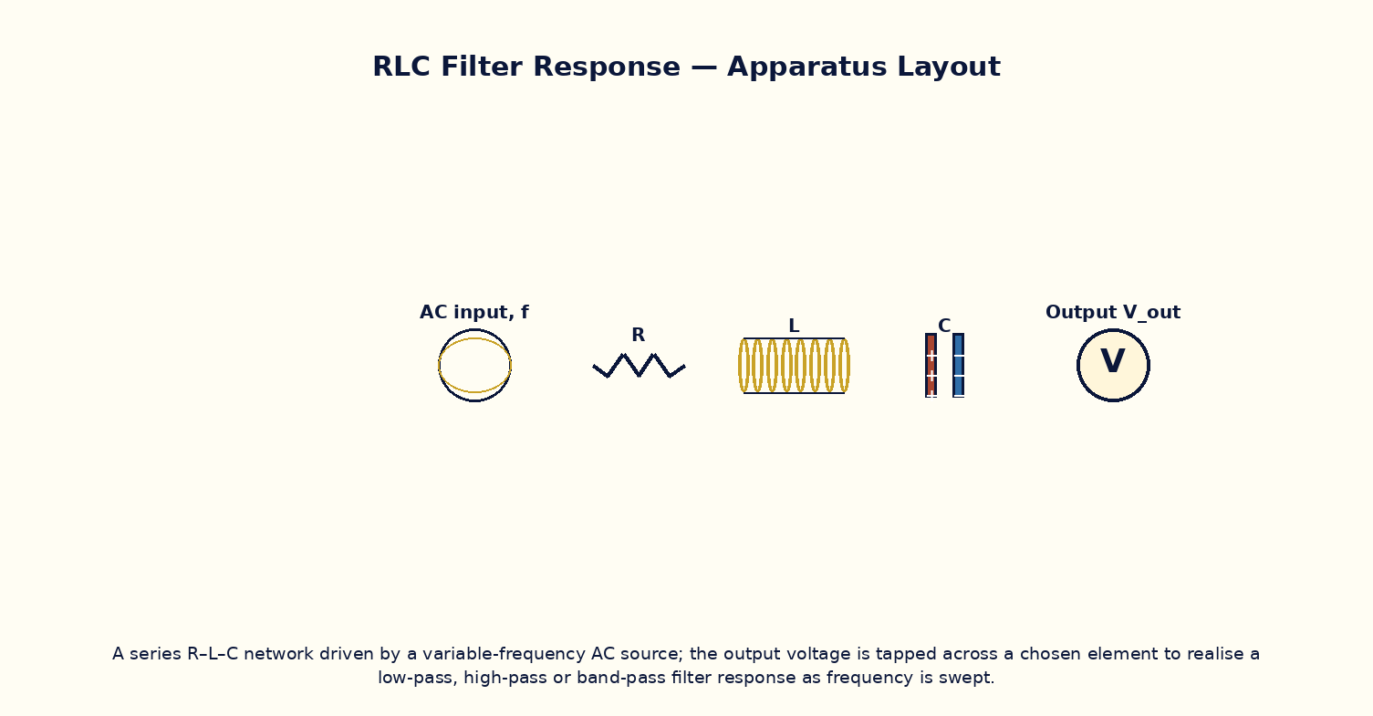
A series combination of a resistor R, inductor L and capacitor C driven by an AC source of variable frequency behaves very differently depending on which element's voltage is taken as the output. Because the inductive reactance ωL grows with frequency while the capacitive reactance 1/ωC falls with frequency, the net series reactance (ωL − 1/ωC) passes through zero at the resonant frequency ω₀ = 1/√(LC), where the impedance is purely resistive and minimum, and the current (and hence the voltage across R) is maximum. Tapping the output across R therefore realises a band-pass filter, peaking at ω₀ and falling off on either side; the sharpness of this peak is set by the circuit's quality factor Q = ω₀L/R. The same RLC network can equally be configured as a low-pass filter (output across C) or a high-pass filter (output across L), since each element's voltage has a different characteristic frequency dependence — this versatility is why RLC networks are the building blocks of analog filter design.

Governing Formula¶

\[ |H(f)|_{bandpass} = \dfrac{R}{\sqrt{R^2 + (\omega L - 1/\omega C)^2}} \]

Symbol	Meaning
\|H(f)\|	band-pass voltage-gain magnitude (dimensionless, 0–1)
R	series resistance (Ω)
L	series inductance (H)
C	series capacitance (F)
ω	angular frequency, ω = 2πf (rad/s)

Interactive Controls¶

Launch the simulator and use the following controls on the RLC Filters — Low-Pass / High-Pass / Band-Pass Frequency Response panel:

Control	Symbol	Range	Default
Resistance	R	1–1000 Ω	100 Ω
Inductance	L	0.1–100 mH	10 mH
Capacitance	C	0.01–10 µF	1 µF
Signal frequency	f	10–20000 Hz	1592 Hz

Procedure¶

Fix R, L, C at their default values and sweep f from 10 Hz to 20 kHz, recording the gain |H(f)| at each step.
Plot |H(f)| versus f and locate the frequency of maximum gain; compare it with the predicted resonance f₀ = 1/(2π√(LC)).
Find the two frequencies on either side of resonance where the gain falls to 1/√2 of its peak value (the −3 dB points), and compute the bandwidth and Q-factor.
Increase R and repeat, observing that the peak becomes broader and shorter (lower Q) as R increases.
Discuss qualitatively how tapping the output across L instead of R would change the shape of the response curve to a high-pass characteristic.

Observation Table¶

| S. No. | f (Hz) | R (Ω) | L (mH) | C (µF) | |H(f)| | |---|---|---|---|---|---|| | | | | | | | | | | | | | | | | | | | | | | | | | | | | | | | | | | |

Graph¶

Gain |H(f)| vs frequency f

Calculations¶

Use the governing formula above with your tabulated observations to compute the required result for each row. Show at least one complete sample calculation with units.

Result¶

| Quantity | Resonant frequency f₀ and Q-factor | Expected value | % deviation | |---|---|---|---|| | | | | |

Precautions¶

Sweep frequency over a wide enough range to clearly capture both sides of the resonance peak.
Keep R, L, C fixed while sweeping only f to trace out a single, clean response curve.
Use a logarithmic frequency axis if the resonance is very sharp (high Q), for clearer visualisation.
Remember that the −3 dB bandwidth is measured at the half-power (1/√2 amplitude) points, not the half-amplitude points.

Maximum Permissible Error¶

\[ \text{Evaluated numerically at each swept frequency; no simple closed-form propagation} \]

The band-pass gain is a non-monomial function of R, L, C and f, so its uncertainty is best explored numerically by perturbing each input in turn rather than via a single algebraic formula.

Viva-Voce Questions¶

Derive the resonant frequency f₀ = 1/(2π√(LC)) for a series RLC circuit.
Define the quality factor Q and explain how it relates to the sharpness of the resonance peak.
Explain how the same RLC network can realise low-pass, high-pass and band-pass responses depending on which element's voltage is tapped.
What is the phase relationship between current and applied voltage exactly at resonance?
Give one practical application of a band-pass RLC filter (e.g. radio tuning circuits).