Dielectric Polarization & the Clausius–Mossotti Relation¶

Apparatus layout diagram for this experiment

Labelled apparatus layout — original illustration prepared for this guide (not a photograph). See the drag-to-rotate 3-D schematic above for a spatial view of the same setup.

3-D apparatus schematic · drag to rotate, scroll to zoom · A virtual slab of dielectric material placed between capacitor plates with a molecular-scale zoom showing individual dipoles aligning under the applied field, plus a control panel for number density N and atomic polarizability α feeding the Clausius–Mossotti calculator.

Aim¶

To study how an external electric field polarizes a dielectric material, relate the macroscopic polarization to the microscopic atomic polarizability using the Clausius–Mossotti relation, and observe the resulting bound charges.

Theoretical Background¶

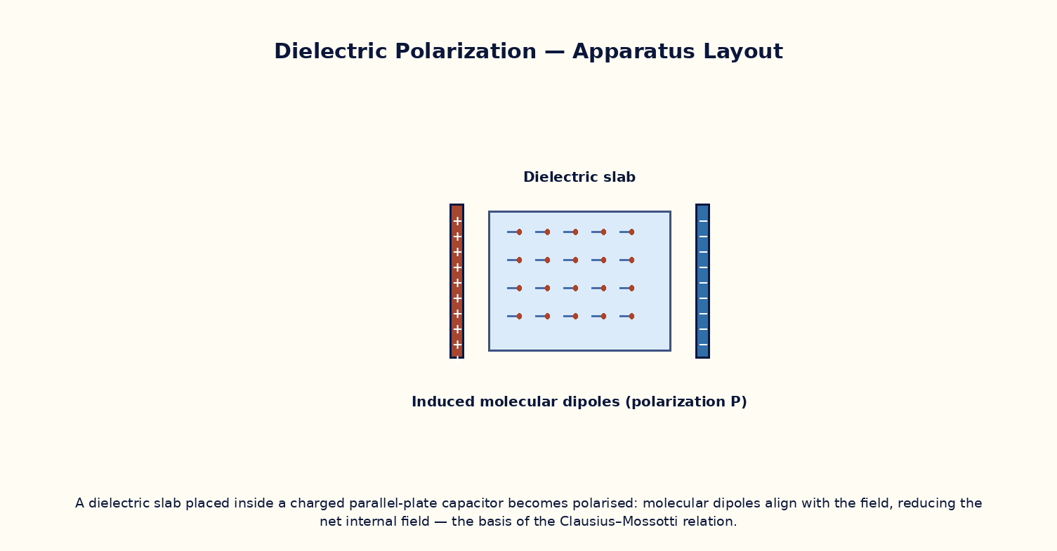
When a dielectric is placed in an external field E, its constituent atoms/molecules develop induced dipole moments (or, for polar molecules, their permanent dipoles partially align), producing a macroscopic polarization P = ε₀χe·E, where χe = εr − 1 is the electric susceptibility. This polarization manifests as bound surface charge σ_b = P·n̂ at the dielectric's surfaces (and bound volume charge where P is non-uniform), which partially cancels the external field inside the material — the origin of the dielectric constant's field-reducing effect seen in the capacitor experiment. The microscopic atomic polarizability α (dipole moment induced per unit local field) is related to the macroscopic εr through the Clausius–Mossotti relation: (εr−1)/(εr+2) = Nα/3ε₀, where N is the number density of polarizable atoms/molecules — this correctly accounts for the fact that each molecule sees not just the applied field but also the field of all the other induced dipoles around it (the local-field correction).

Governing Formula¶

\[ P = ε₀(εr−1)E, (εr−1)/(εr+2) = Nα/(3ε₀) \]

Symbol	Meaning
P	macroscopic polarization (C/m²)
εr	relative permittivity (dielectric constant)
E	applied macroscopic field (V/m)
N	number density of molecules (m⁻³)
α	molecular polarizability (C·m²/V)

Interactive Controls¶

Launch the simulator and use the following controls on the Dielectric Polarization & the Clausius–Mossotti Relation panel:

Control	Symbol	Range	Default
Number density	N	1–50 ×10²⁸ m⁻³	20 ×10²⁸ m⁻³
Molecular polarizability	α	1–50 ×10⁻⁴⁰ C·m²/V	15 ×10⁻⁴⁰ C·m²/V
Applied field	E	1–100 kV/m	20 kV/m

Procedure¶

For a chosen N and α, use the Clausius–Mossotti relation to compute εr, and verify it against the simulator's directly-modelled dielectric response.
Increase N (denser material) and observe εr rising, eventually approaching the 'polarization catastrophe' limit where Nα/3ε₀ → 1.
At fixed N, α, apply an external field E and read off the induced polarization P; verify P = ε₀(εr−1)E.
Zoom into the molecular view and observe individual dipoles growing (or aligning, for polar molecules) proportionally with E.
Compute the bound surface charge density σ_b = P at the dielectric's outer faces and compare it with the field-reduction observed in the parallel-plate-capacitor experiment.
Compare the Clausius–Mossotti prediction with the simpler (and less accurate at high Nα) approximation εr − 1 ≈ Nα/ε₀ that ignores the local-field correction.

Observation Table¶

| S. No. | N (×10²⁸ m⁻³) | α (×10⁻⁴⁰ C·m²/V) | εr (Clausius–Mossotti) | Applied field E (kV/m) | Polarization P (μC/m²) | |---|---|---|---|---|---|| | | | | | | | | | | | | | | | | | | | | | | | | | | | | | | | | | | |

Graph¶

Dielectric Constant vs Number Density N — εr rises steeply as Nα/3ε₀ → 1

15×15 grid — choose your own scale per square; plot from your observation table. Expected trend: εr rises steeply as Nα/3ε₀ → 1

Calculations¶

Use the governing formula above with your tabulated observations to compute the required result for each row. Show at least one complete sample calculation with units.

Result¶

| Case | εr computed | Bound charge σ_b | Remarks | |---|---|---|---|| | | | | |

Precautions¶

Keep Nα/3ε₀ below 1 for a physically stable dielectric; values approaching or exceeding 1 signal the (unphysical, in this simple model) polarization catastrophe/ferroelectric-like instability.
Distinguish clearly between the macroscopic applied field E and the larger local field seen by each individual molecule.
Vary only one of N, α, E at a time when tabulating results.
Remember bound charges are real charges bound to atoms, distinct from free charges on the capacitor plates.

Maximum Permissible Error¶

\[ via Clausius–Mossotti; Δεr estimated numerically from ΔN/N + Δα/α \]

εr is a nonlinear function of Nα, so its propagated error is evaluated numerically from the fractional errors of N and α rather than a simple closed form.

Viva-Voce Questions¶

Define polarization P and relate it to the electric susceptibility χe.
Derive the Clausius–Mossotti relation, explaining the role of the local (Lorentz) field correction.
What is meant by 'bound charge', and where does it appear on/in a polarized dielectric?
Why does the simple relation εr−1 ≈ Nα/ε₀ (without the local-field correction) become inaccurate at high densities?
How does the Clausius–Mossotti relation connect to the Lorentz–Lorenz relation for the refractive index?
Explain qualitatively what a 'polarization catastrophe' represents physically (link to ferroelectricity).