Gauss's Law — Electric Flux Through Closed Surfaces¶

Apparatus layout diagram for this experiment

Labelled apparatus layout — original illustration prepared for this guide (not a photograph). See the drag-to-rotate 3-D schematic above for a spatial view of the same setup.

3-D apparatus schematic · drag to rotate, scroll to zoom · A virtual charge enclosed within a draggable/resizable Gaussian surface (sphere, cube or cylinder); the simulator numerically integrates E·dA over the chosen surface and displays the running flux total.

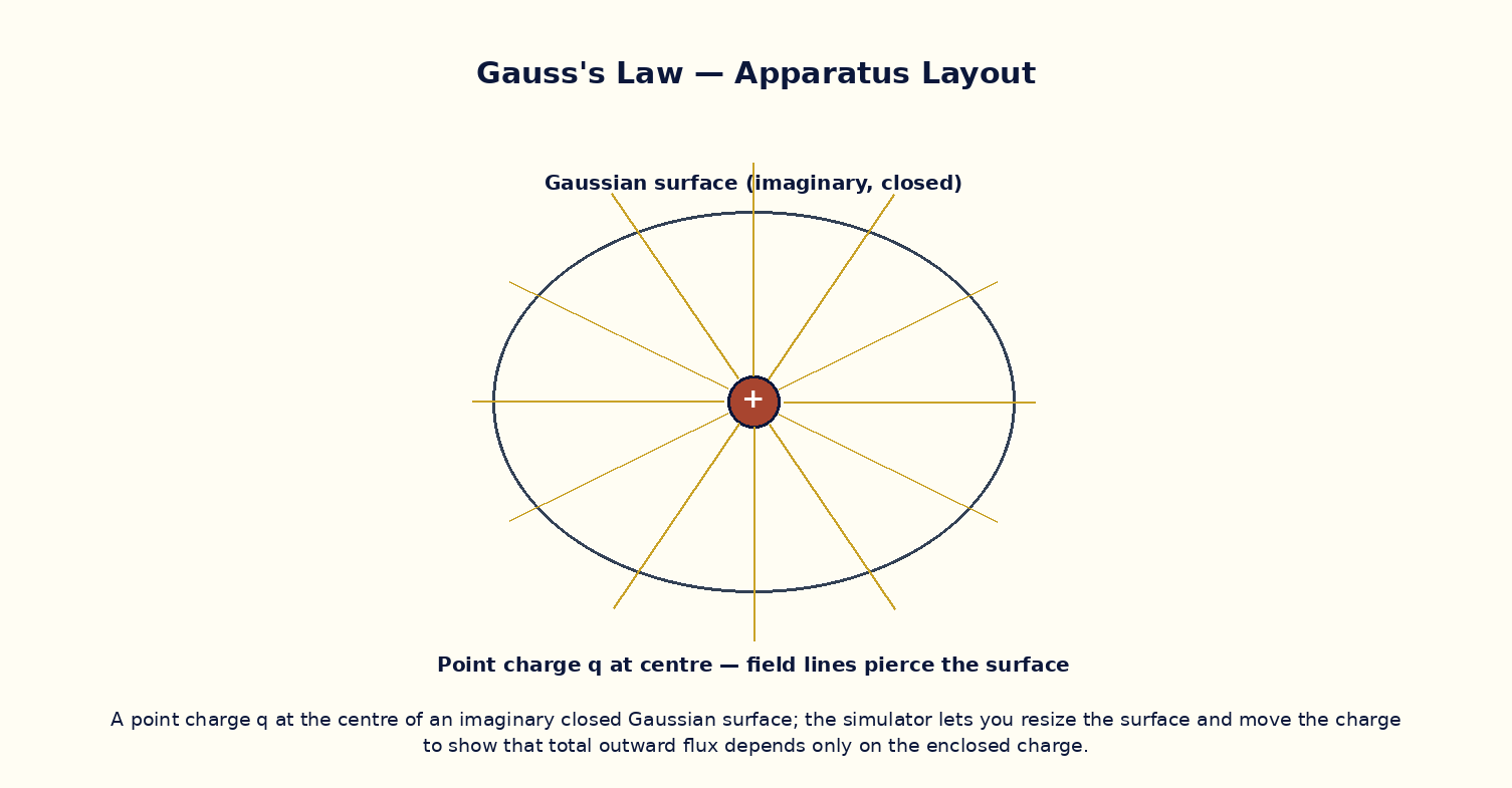
Aim¶

To verify Gauss's law by computing the net electric flux through virtual closed Gaussian surfaces (sphere, cube, cylinder) enclosing a known charge, and to relate the flux to the field of standard symmetric charge distributions.

Theoretical Background¶

Gauss's law states that the net electric flux Φ_E through any closed surface equals the enclosed charge divided by ε₀: Φ_E = ∮ E·dA = Q_enc/ε₀. This holds regardless of the surface's shape and regardless of where the enclosed charge sits inside it, and charges outside the surface contribute zero net flux. For distributions with sufficient symmetry (spherical, cylindrical, planar), Gauss's law lets the field be obtained directly without integrating Coulomb's law: a spherical shell of charge Q gives E = kQ/r² outside and E = 0 inside; an infinite line charge of linear density λ gives E = λ/(2πε₀ρ); an infinite charged sheet of surface density σ gives a uniform field E = σ/(2ε₀) independent of distance from the sheet.

Governing Formula¶

\[ Φ_E = ∮ E·dA = Q_enc / ε₀ \]

Symbol	Meaning
Φ_E	net electric flux through the closed surface (N·m²/C)
Q_enc	total charge enclosed by the surface (C)
ε₀	permittivity of free space

Interactive Controls¶

Launch the simulator and use the following controls on the Gauss's Law — Electric Flux Through Closed Surfaces panel:

Control	Symbol	Range	Default
Enclosed charge	Q_enc	-20–20 nC	10 nC
Charge placed outside surface	Q_out	-20–20 nC	5 nC
Gaussian sphere radius	R	5–40 cm	15 cm
Surface shape	shape	–	sphere

Procedure¶

Place a known charge Q_enc at the centre of a spherical Gaussian surface of radius R and record the computed flux.
Change R (keeping Q_enc fixed) and verify the flux is independent of the radius chosen.
Move Q_enc off-centre within the same surface and confirm the total flux is unchanged.
Add a second charge Q_out entirely outside the surface and verify it contributes zero net flux, even though it changes the local field at the surface.
Switch the Gaussian surface shape from sphere to cube to cylinder (same enclosed charge) and confirm the flux total is identical in every case.
Use the flux value to back-calculate E for a spherical shell and compare with the Coulomb's-law field at the same radius.

Observation Table¶

| S. No. | Surface shape | Q_enc (nC) | Q_out (nC) | Computed flux Φ (N·m²/C) | Q_enc/ε₀ (theory) | |---|---|---|---|---|---|| | | | | | | | | | | | | | | | | | | | | | | | | | | | | | | | | | | |

Graph¶

Field of a Charged Sphere: E vs r — E=0 inside, E∝1/r² outside

15×15 grid — choose your own scale per square; plot from your observation table. Expected trend: E=0 inside, E∝1/r² outside

Calculations¶

Use the governing formula above with your tabulated observations to compute the required result for each row. Show at least one complete sample calculation with units.

Result¶

| Case | Flux measured | Flux predicted (Q_enc/ε₀) | % deviation | |---|---|---|---|| | | | | |

Precautions¶

Make sure the chosen surface is genuinely closed (no gaps) before reading off the flux, or the numerical integration will be inaccurate.
Distinguish carefully between charges enclosed by the surface and charges merely near it but outside.
For the cylindrical surface, remember to include the flux through the flat end-caps as well as the curved side.
Keep the enclosed charge exactly at stated positions when comparing symmetric vs asymmetric placements.

Maximum Permissible Error¶

\[ ΔΦ/Φ = ΔQ_enc/Q_enc \]

Since Φ = Q_enc/ε₀ with ε₀ an exact constant, the fractional error in flux equals the fractional error in the enclosed charge measurement.

Viva-Voce Questions¶

State Gauss's law and explain why it is a direct consequence of Coulomb's law and the inverse-square dependence.
Why is Gauss's law most useful only for highly symmetric charge distributions?
Show that the field inside a uniformly charged spherical shell is exactly zero.
Derive the field of an infinite charged sheet using Gauss's law with a pillbox surface.
If a charge lies exactly on the Gaussian surface, how should it be treated?
How does Gauss's law extend to Gauss's law for magnetism (∇·B = 0), and what does that imply physically?