Magnetic Vector Potential of a Current Loop (Dipole Limit)¶

Apparatus layout diagram for this experiment

Labelled apparatus layout — original illustration prepared for this guide (not a photograph). See the drag-to-rotate 3-D schematic above for a spatial view of the same setup.

3-D apparatus schematic · drag to rotate, scroll to zoom · A small circular current loop of radius a carrying current I, viewed as a magnetic dipole; the vector potential A and field B are evaluated at a distant field point specified by spherical coordinates (r, θ).

Aim¶

To evaluate the magnetic vector potential A of a small current loop in the far-field (magnetic dipole) approximation, and relate its spatial dependence to the resulting dipole field B = ∇ × A.

Theoretical Background¶

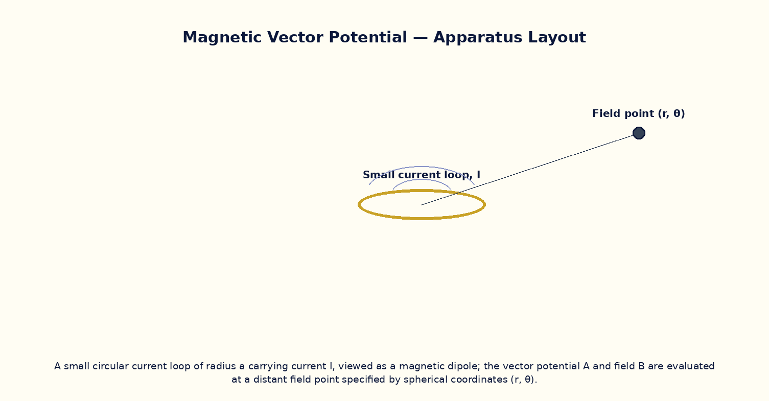
Unlike the scalar electrostatic potential, the magnetic field is more naturally described through a vector potential A, defined by B = ∇ × A, which automatically guarantees ∇·B = 0. For a small planar current loop of radius a carrying current I, viewed from a distance r ≫ a, the vector potential has only an azimuthal component A_φ that falls off as 1/r² and depends on the polar angle θ measured from the loop's axis. This is the magnetic analogue of the electric dipole potential, and the loop's magnetic moment m = I·πa² plays the role that the electric dipole moment p plays in electrostatics. Taking the curl of A_φ reproduces the familiar magnetic dipole field pattern, with field lines emerging from one face of the loop and curving back to enter the other — identical in form to the electric dipole field lines, but without any true magnetic monopoles at the ends.

Governing Formula¶

\[ A_\varphi(r,\theta) = \dfrac{\mu_0 I a^2 \sin\theta}{4 r^2} \]

Symbol	Meaning
A_φ	azimuthal component of the vector potential (T·m)
I	current in the loop (A)
a	loop radius (m)
r	distance to the field point, r ≫ a
θ	polar angle from the loop's axis
μ₀	permeability of free space

Interactive Controls¶

Launch the simulator and use the following controls on the Magnetic Vector Potential of a Current Loop (Dipole Limit) panel:

Control	Symbol	Range	Default
Loop current	I	0.1–10 A	2 A
Loop radius	a	0.5–5 cm	2 cm
Field point distance	r	10–80 cm	30 cm
Polar angle from loop axis	θ	0–180 deg	90 deg

Procedure¶

Fix I = 2 A, a = 2 cm and θ = 90° (equatorial plane), and vary r from 10 cm to 80 cm, recording A_φ.
Plot log A_φ versus log r and verify a slope of −2, confirming the dipole 1/r² fall-off.
Fix r and vary θ from 0° to 180°, and verify that A_φ follows a sinθ dependence, vanishing on-axis (θ = 0° or 180°).
Vary the loop current I and confirm A_φ ∝ I.
Compute the loop's magnetic moment m = Iπa² and compare the measured A_φ(r,90°) with the standard dipole formula A = μ₀m/(4πr²).

Observation Table¶

| S. No. | r (cm) | θ (deg) | I (A) | A_φ (×10⁻⁶ T·cm) | log r | log A_φ | |---|---|---|---|---|---|---|| | | | | | | | | | | | | | | | | | | | | | | | | | | | | | | | | | | | | | | | |

Graph¶

log A_φ vs log r (slope method)

Calculations¶

Use the governing formula above with your tabulated observations to compute the required result for each row. Show at least one complete sample calculation with units.

Result¶

| Quantity | Slope of log A_φ vs log r | Expected value | % deviation | |---|---|---|---|| | | | | |

Precautions¶

Keep r large compared with a to remain within the dipole (far-field) approximation.
Vary only one of I, a, r, θ at a time while tabulating other quantities.
Remember A_φ vanishes exactly on the loop's axis (θ = 0°, 180°) — do not mistake this for an error.
Keep the current direction consistent so that the sign of A_φ has a well-defined meaning.

Maximum Permissible Error¶

\[ \dfrac{\Delta A}{A} = \dfrac{\Delta I}{I} + 2\dfrac{\Delta a}{a} + 2\dfrac{\Delta r}{r} \]

A_φ ∝ Ia²/r² has a and r both squared, each contributing a factor of 2 to the fractional error.

Viva-Voce Questions¶

Why is the magnetic field described using a vector potential rather than a scalar potential?
Define the magnetic dipole moment of a current loop and state its units.
Show qualitatively how B = ∇ × A reproduces the dipole field pattern from A_φ.
Compare the r-dependence and angular dependence of A_φ with the electric dipole potential V.
Why does A_φ vanish on the axis of the loop even though B does not?