RC and RL Transient Circuits — Charging & Discharging
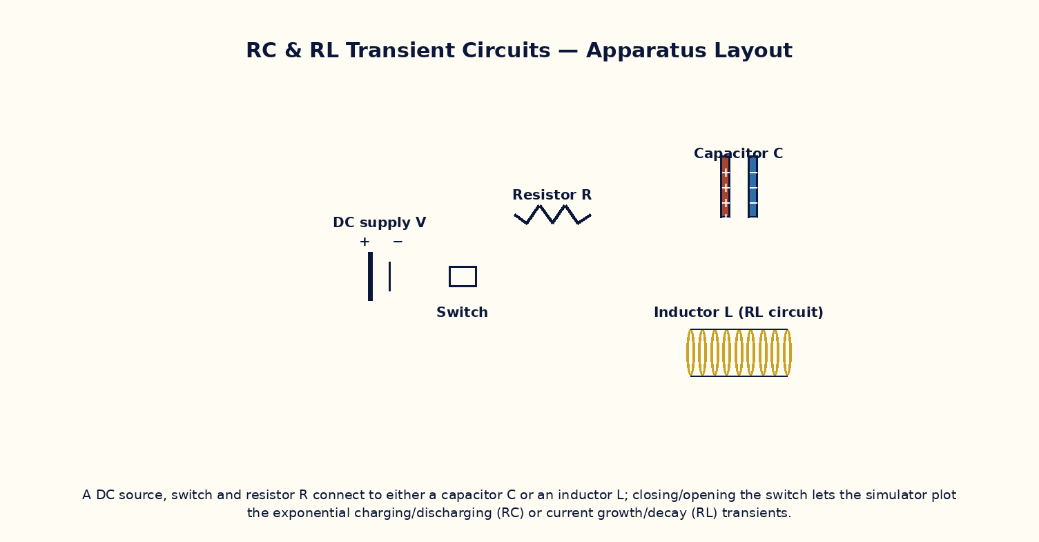
Aim
To study the exponential charging and discharging behaviour of RC and RL circuits, measure the time constant in each case, and verify its dependence on the circuit parameters.
Theoretical Background
In a series RC circuit charged through a resistor R from a battery of EMF ε₀, the capacitor voltage grows as V_C(t) = ε₀(1 − e^{−t/τ}) with time constant τ = RC, and discharges as V_C(t) = V₀ e^{−t/τ} once the battery is removed and the capacitor is shorted through R. Analogously, in a series RL circuit the current grows as I(t) = (ε₀/R)(1 − e^{−t/τ}) with time constant τ = L/R, and decays as I(t) = I₀ e^{−t/τ} when the source is removed. In both cases τ is the time for the quantity to reach (1 − 1/e) ≈ 63.2% of its final value while charging, or to fall to 1/e ≈ 36.8% of its initial value while discharging, and after about 5τ the transient is essentially complete.
Governing Formula
| Symbol | Meaning |
|---|---|
| τ | time constant of the circuit (s) |
| R | resistance (Ω) |
| C | capacitance (F) |
| L | inductance (H) |
| ε₀ | source EMF (V) |
Interactive Controls
Launch the simulator and use the following controls on the RC and RL Transient Circuits — Charging & Discharging panel:
| Control | Symbol | Range | Default |
|---|---|---|---|
| Resistance | R | 1–100 kΩ | 10 kΩ |
| Capacitance | C | 1–100 μF | 10 μF |
| Inductance (RL mode) | L | 0.1–10 H | 1 H |
| Source EMF | ε₀ | 1–20 V | 10 V |
| Circuit (0=RC, 1=RL) | mode | 0–1 | 0 |
Procedure
- For the RC circuit, close the switch and record V_C(t) on the oscilloscope; read off the time to reach 63.2% of ε₀ and compare with RC.
- Vary R (keeping C fixed) and verify τ scales proportionally; repeat varying C at fixed R.
- Discharge the capacitor through R and verify the decay time constant matches the charging time constant.
- Switch to the RL circuit and repeat: measure the growth time constant and verify τ = L/R.
- Vary L and R independently for the RL circuit and verify the corresponding scaling of τ.
- Compare the general shapes of the RC-charging and RL-growth curves and note they are functionally identical apart from which quantity (voltage vs current) is plotted.
Observation Table
| S. No. | Circuit type | R (kΩ) | C (μF) or L (H) | Measured τ (ms) | Calculated τ = RC or L/R (ms) | |---|---|---|---|---|---|| | | | | | | | | | | | | | | | | | | | | | | | | | | | | | | | | | | |
Graph
Capacitor Charging Curve — 63.2% at t=τ, ~99% at t=5τ
Calculations
Use the governing formula above with your tabulated observations to compute the required result for each row. Show at least one complete sample calculation with units.
Result
| Circuit | τ measured | τ calculated | % deviation | |---|---|---|---|| | | | | |
Precautions
- Allow at least 5τ for the transient to settle before considering the circuit to be at steady state.
- Discharge the capacitor completely (or de-energize the inductor) before starting a fresh charging run.
- Vary only R or only C (or only L) between successive runs to isolate each dependence.
- Remember an ideal inductor's current cannot change instantaneously, and an ideal capacitor's voltage cannot change instantaneously — use this as a sanity check on the simulated traces.
Maximum Permissible Error
τ = RC is a simple product, so fractional errors in R and C add directly.
Viva-Voce Questions
- Derive the charging equation of an RC circuit from Kirchhoff's voltage law.
- What is the physical significance of the time constant τ, and how is it read off an exponential curve graphically?
- Why do the RC-charging and RL-growth curves have the same mathematical form?
- How much energy is ultimately stored in the capacitor after full charging, and how does this compare with the energy dissipated in R during charging?
- What happens to the time constant if R is doubled while C is halved?
- Explain the duality between RC and RL transient circuits in terms of the roles of voltage and current.