Electric Field & Potential Due to an Electric Dipole
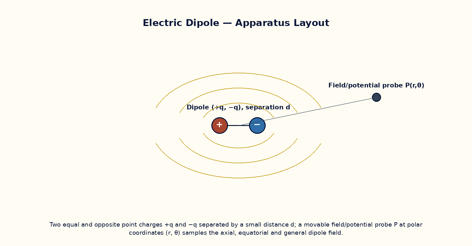
Aim
To compute and plot the electric field and potential of an electric dipole along its axial and equatorial lines, and to study the angular variation of the field at a fixed distance.
Theoretical Background
An electric dipole consists of two equal and opposite charges +q and −q separated by a small distance 2a, with dipole moment p = q·(2a) directed from −q to +q. For distances r ≫ a, the potential at a point making angle θ with the dipole axis is V = p·cosθ/(4πε₀r²), and the field has a radial component E_r = 2p·cosθ/(4πε₀r³) and a tangential component E_θ = p·sinθ/(4πε₀r³). On the axial line (θ = 0) the field is E_axial = 2kp/r³, twice the equatorial-line field E_equatorial = kp/r³ (θ = 90°), and the two fields are oppositely directed relative to p. This 1/r³ falloff (steeper than the 1/r² of a point charge) is a signature of the dipole and is the basis for understanding polar-molecule interactions and dielectric polarization.
Governing Formula
| Symbol | Meaning |
|---|---|
| p | dipole moment, p = q·2a (C·m) |
| r | distance from the dipole centre (m) |
| θ | angle from the dipole axis |
| k | 1/4πε₀ = 8.988×10⁹ N·m²/C² |
Interactive Controls
Launch the simulator and use the following controls on the Electric Field & Potential Due to an Electric Dipole panel:
| Control | Symbol | Range | Default |
|---|---|---|---|
| Charge magnitude | q | 1–20 nC | 5 nC |
| Charge separation | 2a | 1–10 cm | 4 cm |
| Probe distance | r | 5–50 cm | 20 cm |
| Probe angle from axis | θ | 0–180 ° | 0 ° |
Procedure
- Set the probe on the axial line (θ = 0°) and record E and V as r is increased from 5 cm to 50 cm.
- Plot log E versus log r for the axial case and verify the slope is −3 (not −2 as for a single point charge).
- Move the probe to the equatorial line (θ = 90°) and confirm V ≈ 0 there at every r.
- At a fixed r = 20 cm, sweep θ from 0° to 180° and tabulate E and V; note the sign reversal of V past θ = 90°.
- Compare the axial field magnitude with the equatorial field magnitude at the same r; verify the 2:1 ratio.
- Increase the separation 2a and confirm the point-dipole formulas remain accurate only while r ≫ a.
Observation Table
| S. No. | θ (°) | r (cm) | Field E (N/C) | Potential V (volt) | log r | log E | |---|---|---|---|---|---|---|| | | | | | | | | | | | | | | | | | | | | | | | | | | | | | | | | | | | | | | | |
Graph
Axial Field E vs r (log-log) — slope ≈ -3
Calculations
Use the governing formula above with your tabulated observations to compute the required result for each row. Show at least one complete sample calculation with units.
Result
| Line | Field formula verified | Slope obtained | Expected slope | |---|---|---|---|| | | | | |
Precautions
- Always keep r ≫ 2a so the point-dipole approximation is valid; note the deviation if this is violated.
- Track the sign of the potential carefully — it is positive on the +q side and negative on the −q side of the equatorial plane.
- When sweeping θ, keep r fixed to isolate the angular dependence cleanly.
- Distinguish clearly between the radial and tangential components of E when off-axis.
Maximum Permissible Error
E_axial = 2kp/r³ with p=q·(2a) varies as r⁻³, so its fractional uncertainty carries a factor of 3 from r.
Viva-Voce Questions
- Why does the dipole field fall off as 1/r³ while a single point charge's field falls off as 1/r²?
- Show that the potential on the equatorial line of a dipole is zero everywhere.
- What is the torque on a dipole placed in a uniform external field, and at what orientation is it maximum?
- Define dipole moment as a vector and state its SI unit.
- How would the field pattern change for a linear quadrupole (two dipoles placed back-to-back)?
- Explain the physical origin of polar molecules' permanent dipole moment (e.g. in water).