Poynting Vector & Power Flow in a Coaxial Cable¶

Apparatus layout diagram for this experiment

Labelled apparatus layout — original illustration prepared for this guide (not a photograph). See the drag-to-rotate 3-D schematic above for a spatial view of the same setup.

3-D apparatus schematic · drag to rotate, scroll to zoom · Cross-section of a coaxial cable carrying DC power between inner and outer conductors; the Poynting vector S = E × H, evaluated in the annular dielectric region, points axially and its integral gives the transmitted power VI.

Aim¶

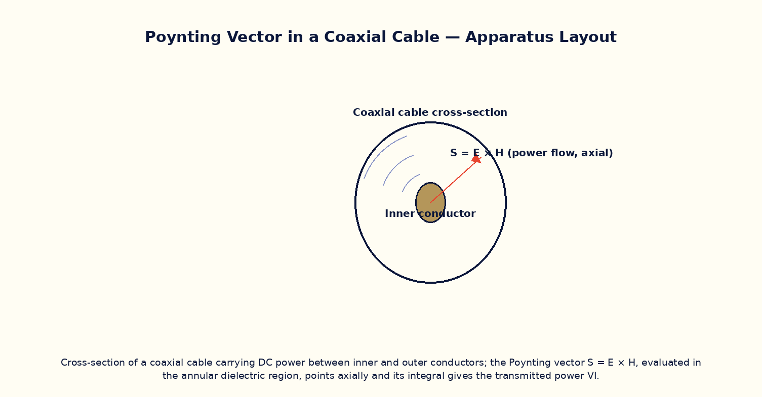
To compute the Poynting vector S = E × H in the dielectric region between the inner and outer conductors of a coaxial cable carrying DC power, and to verify that its integral over the annular cross-section reproduces the transmitted electrical power P = VI.

Theoretical Background¶

It is a common misconception that electrical power flows through the metal of a wire; in fact, according to Poynting's theorem, electromagnetic power flows through the space (the dielectric or vacuum) surrounding the conductors, described by the Poynting vector S = E × H, with the conductors merely guiding the fields. In a coaxial cable carrying a steady current I at voltage V, the radial electric field E between the inner conductor (radius a) and outer shield (radius b) is set up by the charge on the conductors, while the azimuthal magnetic field H circles the inner conductor according to Ampere's law. Their cross product S = E × H points purely in the axial direction, along the cable, and integrating S over the annular cross-sectional area between a and b reproduces exactly the transmitted power P = VI — a striking and non-obvious confirmation that the field-based picture of energy flow is fully consistent with the familiar circuit-theory result.

Governing Formula¶

\[ S(r) = \dfrac{VI}{2\pi r^2 \ln(b/a)} \]

Symbol	Meaning
S(r)	axial Poynting flux at radius r (W/m²)
V	voltage between inner and outer conductors (V)
I	current carried by the conductors (A)
a	inner-conductor radius (m)
b	outer-conductor (shield) radius (m)
r	field-point radius, a < r < b

Interactive Controls¶

Launch the simulator and use the following controls on the Poynting Vector & Power Flow in a Coaxial Cable panel:

Control	Symbol	Range	Default
Conductor voltage	V	1–400 V	100 V
Conductor current	I	0.1–20 A	5 A
Inner-conductor radius	a	0.3–5 mm	1 mm
Outer-conductor (shield) radius	b	2–20 mm	5 mm
Field point radius (a<r<b)	r	1–19 mm	2.5 mm

Procedure¶

Fix V, I, a, b at their default values and vary the field-point radius r from just above a to just below b, recording S(r) at each step.
Plot S versus r and verify the expected 1/r² fall-off across the annular gap.
Numerically (or graphically) integrate S(r) over the annular cross-section (2πr·dr from a to b) and compare the result with the transmitted power P = VI.
Vary V and I in turn and verify that S(r) at any fixed r scales linearly with each.
Discuss why S is zero for r < a or r > b (inside the inner conductor or outside the shield).

Observation Table¶

| S. No. | r (mm) | V (V) | I (A) | S(r) (kW/m²) | |---|---|---|---|---|| | | | | | | | | | | | | | | | | | | | | | | | | | | | | | |

Graph¶

Poynting flux S vs radius r

Calculations¶

Use the governing formula above with your tabulated observations to compute the required result for each row. Show at least one complete sample calculation with units.

Result¶

| Quantity | ∫ S · dA over annulus (→ compare with VI) | Expected value | % deviation | |---|---|---|---|| | | | | |

Precautions¶

Only evaluate S(r) strictly between the inner and outer conductors (a < r < b); the field, and hence S, is zero elsewhere in an ideal coaxial cable.
Keep the current steady (DC) so the simple electrostatic-plus-magnetostatic picture applies without radiation effects.
Use consistent SI units when integrating S(r) over the annular area to compare with VI.
Vary only one of V, I, a, b, r at a time while tabulating.

Maximum Permissible Error¶

\[ \dfrac{\Delta S}{S} = \dfrac{\Delta V}{V} + \dfrac{\Delta I}{I} + 2\dfrac{\Delta r}{r} \]

S(r) ∝ VI/r² has r squared in the denominator, contributing a factor of 2 to the fractional error.

Viva-Voce Questions¶

State Poynting's theorem and define the Poynting vector.
Explain the common misconception that power flows 'through the wire', and how the Poynting-vector picture corrects it.
Why does S point purely axially in a coaxial cable carrying steady current?
Show that integrating S over the annular cross-section reproduces P = VI.
How would the picture change for an AC (time-varying) signal instead of DC?