Method of Images — Charge Near a Grounded Conducting Plane¶

Apparatus layout diagram for this experiment

Labelled apparatus layout — original illustration prepared for this guide (not a photograph). See the drag-to-rotate 3-D schematic above for a spatial view of the same setup.

3-D apparatus schematic · drag to rotate, scroll to zoom · A point charge +q is held at height d above an infinite grounded conducting plane; the induced surface charge distribution and the attractive force are exactly equivalent to those of an image charge −q placed a mirrored distance d below the plane.

Aim¶

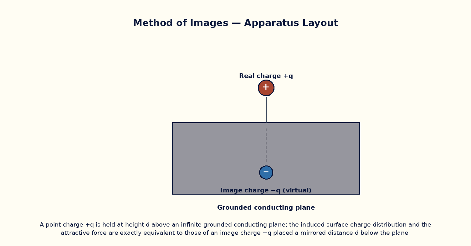
To use the method of images to compute the attractive force between a point charge and a nearby infinite grounded conducting plane, and to show that this force equals that between the real charge and an equal-and-opposite image charge at the mirror position.

Theoretical Background¶

When a point charge q is placed near a grounded conducting plane, the plane's free electrons rearrange themselves so that the plane remains at zero potential everywhere on its surface. Solving this boundary-value problem directly is difficult, but the method of images gives an elegant shortcut: for the region above the plane, the actual field is identical to the field that would be produced by the real charge q together with a fictitious image charge −q placed at the mirror-image position, with the conducting plane removed entirely. Because both configurations satisfy Laplace's equation above the plane and both give V = 0 on the plane, the uniqueness theorem guarantees they produce the same field in that region. The charge is therefore attracted towards the plane exactly as it would be attracted towards a real charge −q at distance 2d, even though no such charge physically exists — the attraction is due entirely to the induced surface charge on the plane.

Governing Formula¶

\[ F = \dfrac{q^2}{4\pi\varepsilon_0 (2d)^2} \]

Symbol	Meaning
F	attractive force on the charge towards the plane (N)
q	magnitude of the point charge (C)
d	perpendicular height of the charge above the plane (m)
ε₀	permittivity of free space

Interactive Controls¶

Launch the simulator and use the following controls on the Method of Images — Charge Near a Grounded Conducting Plane panel:

Control	Symbol	Range	Default
Point charge	q	1–50 nC	12 nC
Height above the grounded plane	d	1–20 cm	5 cm

Procedure¶

Set the charge q = 12 nC and vary the height d from 1 cm to 20 cm in steps of 1 cm, recording the computed attractive force F at each step.
Plot log F versus log d; the slope should equal −2, confirming the inverse-square dependence on d (equivalently on the image separation 2d).
Fix d = 5 cm and vary q from 5 nC to 50 nC, verifying that F is proportional to q².
Compare the force at a given d with the force computed from Coulomb's law between two real charges q and −q separated by 2d, and confirm they are numerically identical.
Discuss what happens to the induced surface charge density directly beneath the point charge as d is decreased.

Observation Table¶

| S. No. | Height d (cm) | Charge q (nC) | Force F (×10⁻⁹ N) | log d | log F | |---|---|---|---|---|---|| | | | | | | | | | | | | | | | | | | | | | | | | | | | | | | | | | | |

Graph¶

log F vs log d (slope method)

Calculations¶

Use the governing formula above with your tabulated observations to compute the required result for each row. Show at least one complete sample calculation with units.

Result¶

| Quantity | Slope of log F vs log d | Expected value | % deviation | |---|---|---|---|| | | | | |

Precautions¶

Treat the plane as a genuinely infinite, grounded conductor — the image-charge method fails near the edges of a finite plane.
Keep the point charge's physical size much smaller than d, so it may be treated as a true point charge.
Vary only one parameter (q or d) at a time when tabulating results.
Remember that the image charge is a mathematical construct valid only in the region above the plane, not below it.

Maximum Permissible Error¶

\[ \dfrac{\Delta F}{F} = 2\dfrac{\Delta q}{q} + 2\dfrac{\Delta d}{d} \]

F ∝ q²/d², so both q and d enter squared and each contributes a factor of 2 to the fractional error.

Viva-Voce Questions¶

State the method of images and explain why it is valid only in the region containing the real charge.
Derive the expression for the force of attraction between the charge and the grounded plane.
How does the induced surface charge density vary with lateral distance from the point directly below the charge?
What would change if the plane were held at a fixed non-zero potential instead of being grounded?
Extend the method of images to the case of a charge between two perpendicular grounded planes.